Note: this is an old post. The updated post series from 2020 is LEAP's 3-Part Series on "What y+ should I use in my simulations?" which is available here:
- Part 1 – Understanding the physics of boundary layers
- Part 2 – Resolving each region of the boundary layer
- Part 3 – Understanding impact of Y+ and number of prism layers on flow resolution
Old Post continues:
In recent posts in our series of Turbulence Modelling posts, we have covered boundary layer theory and touched on some useful meshing and post-processing guidelines to check you are appropriately resolving the boundary layer profile. Today we will consider three critical questions that are often asked by CFD engineers when developing or refining a CFD simulation:
- Am I using the correct turbulence model for the type of results I am looking for?
- Do I have an appropriate Y+ value and a sufficient number of inflation layers?
- Am I using the right wall function for my problem?
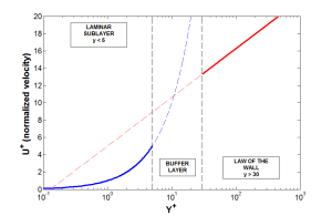
This topic is so important because we know that in turbulent flows the velocity fluctuations within the turbulent boundary layer can be a significant percentage of the mean flow velocity, so it is critical that we capture these effects with accuracy. A Reynolds averaging approach using turbulence models will provides us with an estimate of the increased levels of stress within the boundary layer, termed the Reynolds stresses. In order to appreciate the use of wall functions and the influence of walls on the turbulent flowfield, we should first gain familiarity with the composite regions of the turbulent boundary layer:
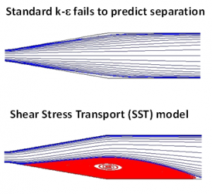
In the laminar sub-layer region (Y+ < 5) inertial forces are less domineering and the flow exhibits laminar characteristics, which is why this is known as the low-Re region. Low-Re turbulent models (e.g. the SST model) aim to resolve this area and therefore require an appropriate mesh resolution to do this with accuracy. This is most critical for flows with a changing pressure gradient where we expect to see separation, as observed below.
In the law of the wall region, inertial forces strongly dominate over viscous forces and we have a high presence of turbulent stresses (this is known as the high-Re composite region). If using a low-Re model, the whole turbulent boundary layer will be resolved including the log-law region. However, it possible to use semi-empirical expressions known as wall functions to bridge the viscosity-affected region between the wall and the fully-turbulent region.
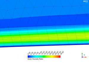
Contours of the eddy viscosity ratio on a low-Re grid illustrating high turbulent viscosity in the log-law region as opposed to the laminar sub-layer
The main benefit of this wall function approach lies in the significant reduction in mesh resolution and thus reduction in simulation time. However, the shortcoming lies in numerical results deteriorating under subsequent refinement of the grid in wall normal direction (thus reducing the Y+ value into the buffer layer zone). Continued reduction of Y+ to below 15 can gradually result in unbounded errors in wall shear stress and wall heat transfer (due to the damping functions inherent within the wall function approach).
Bearing all of the above in mind, and keeping our eye on finding the right balance between accuracy, stability and speed, we can tackle a wide variety of CFD problems using the following guidelines:
What results am I interested in and am I using the right turbulence model?
If our aim is to accurately predict the boundary layer velocity or thermal profile, or if the developing boundary layer will tend to separate (due to a changing pressure gradient – and not because of sharp edges or discontinuities in the geometry), then we recommend the use of a low-Re model. Low-Re models are also required for accurate pressure-drop or drag calculations. We highly recommend the use of the Shear Stress Transport (SST) model, but all ω-based models or ε-based models with enhanced wall treatment may be used. For high speed external aerodynamic flows, the one-equation Spalart-Allmaras model (with Y+ < 2) may also be considered to reduce the computational time. Alternatively, for flows where wall-bounded effects are not a priority, or if separation is expected to occur only due to sharp changes in the geometry, an ε-based wall function approach is more than sufficient. In ANSYS CFD, all ω-based models and the SST model are capable of resorting to a wall function formulation (automatic wall treatment) in the presence of coarse mesh resolutions near the wall without any further user input. Wall function models are also useful for calibrating our CFD models, due to the decreased simulation time.
What is my Y+ value and do I have a sufficient number of prism layers?
When using low-Re models or any models with enhanced wall treatment, the average Y+ value should be on the order of ~1 to ensure we are capturing the laminar sub-layer. When using wall function models, the Y+ value should ideally be above 15 to avoid erroneous modelling in the buffer layer and the laminar sub-layer. High quality numerical results for the boundary layer will only be obtained if the overall resolution of the boundary layer is sufficient. This requirement in some cases is more important than achieving certain Y+ values. The minimum number of cells to cover a boundary layer accurately is around 10, but values of 20 are desirable. The total thickness of the prisms should be implemented such that around 15 or more nodes are actually covering the boundary layer. Our next post in this series on the turbulent boundary layer will cover a very useful and practical technique to post-process the resolution of the boundary layer, and offer insight into modifications required to improve accuracy.
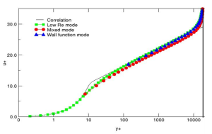
Boundary layer velocity profile modeled with standard k-e for three different mesh densities using Enhanced Wall Treatment
Am I using the right wall function?
In ANSYS CFD, all turbulence models are y-plus independent. However selecting the most appropriate wall function is dependent on level of refinement of our wall adjacent mesh, or the relative scales in our flow. Use of the standard wall function (ε-based models) implies that our boundary layer mesh lies entirely within the log-law region of the boundary layer. For industrial applications, this in fact might be difficult to achieve due to varying geometrical and velocity scales associated with our model – and therefore grids inherently designed with arbitrary refinement. We highly recommend the use of the scalable wall function, which offers an elegant solution to this ambiguity often encountered. This wall function virtually displaces the mesh to a Y+ ~ 11.225 (transition to the log-law composite layer) irrespective of the level of refinement, thereby avoiding the erroneous modelling of the laminar sub-layer and buffer region. It is also important to note that for grids designed with a Y+ > 11.225, the scalable wall function will provide identical results to the standard wall function. Enhanced wall treatment may further be selected for ε-based models on refined low-Re grids, and is also formulated such that it can perform well for meshes of intermediate resolution. However the use of enhanced (or non-equilibrium) wall treatment for low-Re modelling of the turbulent boundary layer is generally not recommended and more confidence in our solution can be obtained by selecting a suitable ω-based formulation, such as the SST model.


