Note: this is an old post. The updated post series from 2020 is LEAP's 3-Part Series on "What y+ should I use in my simulations?" which is available here:
- Part 1 – Understanding the physics of boundary layers
- Part 2 – Resolving each region of the boundary layer
- Part 3 – Understanding impact of Y+ and number of prism layers on flow resolution
Old Post continues:
Previously we have discussed the importance of an inflation layer mesh and how to implement one easily in ANSYS Meshing. We also touched upon the concept of mesh y+ values and how we can estimate them during the inflation meshing process. In other posts, we also discuss the different turbulence models and eddy simulation methods available to ANSYS CFD users. In today's post, we'll talk in more detail about y+ values apply to the most commonly used turbulence models.
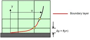
From our earlier discussions, we now understand that the placement of the first node in our near-wall inflation mesh is very important. The y+ value is a non-dimensional distance (based on local cell fluid velocity) from the wall to the first mesh node, as you can see in the image below. To use a wall function approach for a particular turbulence model with confidence, we need to ensure that our y+ values are within a certain range.
Looking at the image above, we need to be careful to ensure that our y+ values are not so large that the first node falls outside the boundary layer region. If this happens, then the Wall Functions used by our turbulence model may incorrectly calculate the flow properties at this first calculation point which will introduce errors into our pressure drop and velocity results. The upper range of applicability will vary depending on the flow physics and the extent of the boundary layer profile.
For instance, flows with very high Reynolds numbers (typically aircraft, ships, etc) will experience a logarithmic boundary layer that extends to several thousand y+ units, whereas low Reynolds number flows such as turbine blades may have an upper limit as little as 100 y+ units. In practice, this means that the use of wall functions for these class of flows should be avoided as their use will limit the overall number of mesh nodes that can be sensibly placed within the boundary layer. In general, it is recommended that you endeavour to place sufficient inflation layer cells within the boundary layer, rather than simply focusing on achieving any particular y+ value. This will be covered in detail in a future post
In addition to the concern about having a mesh with y+ values that are too large, you need to be aware that if the y+ value is too low then the first calculation point will be placed in the viscous sublayer (logarithmic) flow region and the Wall Functions will also be outside their validity (below about y+ < 11). You can imagine that this would become an issue if a mesh intended to be used with wall functions is then refined near the wall. Fortunately, the use of scalable wall functions in ANSYS CFD products now takes care of these problems and produces consistent results for grids of varying y+. Without any further user involvement, the scalable wall functions activate the local usage of the log law in regions where the y+ is sufficiently small, in conjunction with the standard wall function approach in coarser y+ regions.
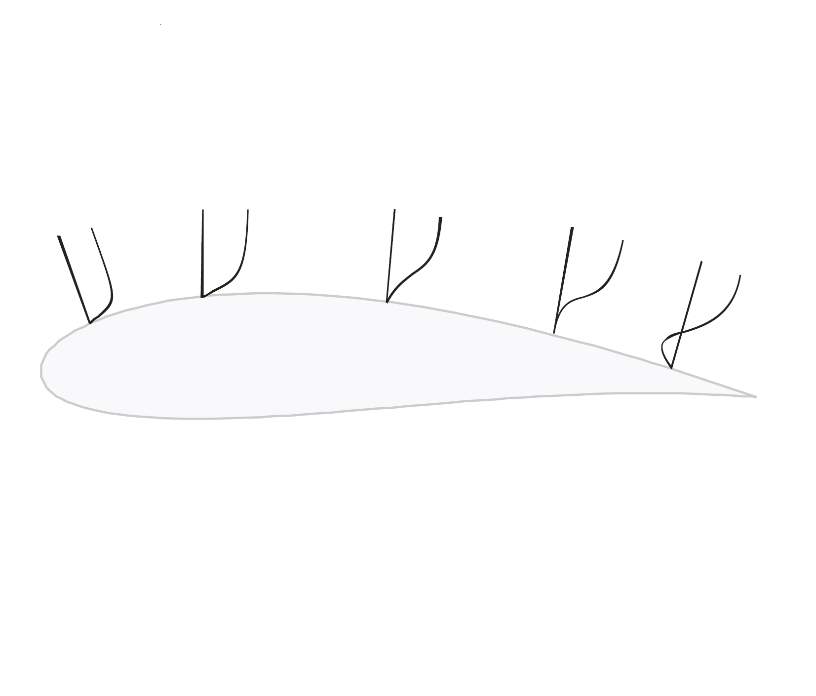
So, where should you start? We have learnt that the wall function approach and y+ value required is determined by the flow behaviour and the turbulence model being used. If you have an attached flow, then generally you can use a Wall Function approach, which means a larger initial y+ value, smaller overall mesh count and faster run times. If you expect flow separation and the accurate prediction of the separation point will have an impact your result, such as the drag or lift forces experienced by the ellipse below, then you would be advised to resolve the boundary layer all the way to the wall with a finer mesh. Please refer to this post for a more detailed explanation of appropriate turbulent wall function and modelling approaches.
Once we know our preferred approach, we can estimate the thickness for our first inflation layer cell using the equation below, which can be used to calculate the distance value for a specific velocity fluid and the required y+ value (based on the flow over a flat plate). This is usually a good initial estimate and the y+ value we aim for will depend on our turbulence model selection.
Note that Δy is the distance of the first node from the wall, L is the flow characteristic length scale, y+ is the desired y+ value, Re_L is the Reynolds Number based on your problem's characteristic length scale.
Unfortunately, as the y+ value is dependent on the local fluid velocity which varies across the wall significantly for most industrial flow applications, it is not possible to know your exact y+ prior to running an initial simulation. For this reason, it is important that you get into the habit of checking your y+ values as part of your normal post-processing in ANSYS CFD-Post so that you can make sure you are in the valid range for your flow physics and turbulence model selection.
Our next post in this series concentrates on the feasibility and selection of different wall functions, based on the applied turbulence modelling strategy.
This is still an area of active research and is a hot topic for many of our CFD users. If you have any questions or comments, please leave a message below or contact our CFD Technical Support team for more detailed technical information on these topics.


