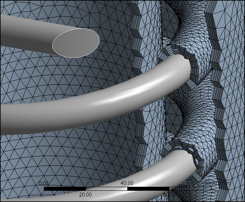
Throughout our first set of Tips & Tricks posts relating to meshing controls and meshing methods, we have made mention of Inflation Layers a number of times. Let's take this opportunity to explain exactly why inflation layers are a critical component of a good CFD mesh and how we can create them easily within ANSYS Meshing.
In our first posts on Mesh Sizing we explained that as well as capturing all key features of the geometry (using local sizing and the curvature size function), we also need to have a sufficiently fine mesh to adequately capture regions where the flow will experience rapid change in key variables such as pressure, velocity or temperature. This initially led us to a better understanding of how we should apply Global and Local Mesh Controls.
Now, if you think about moving a probe from the freestream flow towards one of the walls in your fluid domain, as you approach the wall you will notice that the velocity decreases non-linearly up to a point where the fluid will have zero velocity at the wall. This is what is termed the "no slip" wall condition in CFD.
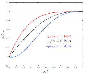
If we plot a typical velocity profile in the near-wall region, we can see that we have a large change in velocity in the wall normal direction and it is important to our CFD simulation that we capture this gradient correctly. To do this, we need to use inflation layer meshing to accurately capture the boundary layer region for any wall-bounded turbulent flows. The image below plots the non-dimensional velocity versus the non-dimensional wall normal distance, with each line from top to bottom demonstrating the difference between a favourable pressure gradient through to adverse pressure gradient with flow separation. It is clear that the flow behaviour in the near wall region is fairly complex and needs to be captured appropriately to have any confidence in our CFD results, especially if we intend to report key engineering data such as separation points or pressure drops.
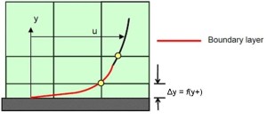
Providing a suitable inflation mesh for the geometry is strongly tied to the choice of the turbulence model, and the flow field we are interested in capturing. We can elect to resolve the complete profile of the boundary layer of alternatively we can make use of empirical wall functions to reduce the cell count (see our post on turbulence modelling and wall functions). If we refer to the images below, on the left hand side we observe that the boundary layer profile is modelled with a reduced cell count, which is characteristic of a wall function approach. On the right, the boundary layer profile is resolved all the way to the wall. This will provide a more accurate resolution of the boundary layer. For certain simulations such as flows with strong wall-bounded effects, this resolution is absolutely necessary. For other simulations, the added computational expense is not always justifiable.
At this point, we begin to understand that the placement of the first node in our near-wall mesh is very important. We use a non-dimensional distance (based on local cell fluid velocity) from the wall to the first node, which we term the y+. To use a wall function approach for a particular turbulence model with confidence, we need to ensure that our y+ values are within a certain range. This topic is covered in detail here
This topic will also be discussed more in a future post, but in general it is considered good practice to include between 10 and 15 inflation layers situated within the boundary layer of your flow to accurately resolve the boundary layer and accurately predict any separation or reattachment points. So now that we understand the importance of inflation layers to our CFD mesh, how can we set them up?
For a 3D body, we begin by choosing the body (typically a fluid domain) that we want to create the inflation mesh within, and then identify the faces that we want to inflate from.
For a swept body, we begin by selecting the source face, and then the boundaries or edges from which we wish to inflate. This is a different approach from other 3D bodies as the source face is meshed first individually, which is then swept through the body.
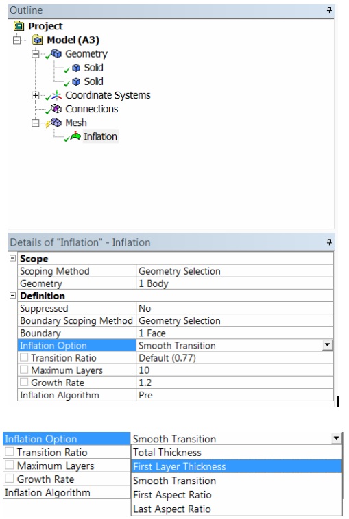
Once we have specified these boundaries to be inflated (either surfaces or edges), then it is easy to define the number of inflation layers, inflation growth rate and select one of the following methods: Total Thickness, First Layer Thickness, First layer Aspect Ratio, Last Layer Aspect Ratio or the Smooth Transition option (which uses a ratio based on the local surface mesh size).
As I mentioned earlier, we find that the First Layer thickness option is the best place to start, especially when you are trying to achieve a particular y+ value as this value can be parametrised in ANSYS Workbench so that any changes to the First Layer Thickness parameter will be proportional to the y+ values that you expect in your solution. The first layer thickness that you choose should be used to obtain the correct y+ value for the turbulence model and flow behaviour that you are dealing with, which we will discuss in a future post.
If you have any questions related to this post or you would like some advice for your own inflation meshing, then please post a comment below or alternatively contact our LEAP ANSYS CFD Support Team.


