Modern designs analysed with the ANSYS Suite of products are complex and often have a significant number of variables which can be tuned to improve the performance of the product. This presents a considerable problem for the design engineer, “how do I work out which variables are the most important?”, and the follow-on question, “how do I tune the variables I have available to achieve an improvement in the product performance?”.
Given unlimited computational resources, every engineering problem would be run hundreds of thousands of times to discover the most optimal design configuration to suit the end use case. Unfortunately, this is very rarely a possibility. With the introduction of cloud computing, the cost of the analysis is charged by the hour which makes minimising the computation required even more of a priority than it was with a traditional workstation. For very simple simulations such as 0-D network analysis, almost 100,000 simulations could be run in a 24-hour period. However, most of the problems that the ANSYS CFD products are used to analyse are considerably more complex in nature. The total number of simulations which can be executed in a 24-hour period if each run requires 20 minutes is just 72.
Brute force is no longer an option so the question now becomes “how do I eliminate as many variables as possible and optimise with a total of just 72 runs?”. ANSYS optiSLang offers a compelling proposition for achieving these goals while simultaneously giving the engineer even more tools for exploring the possible performance envelope within the design parameters.
De-sensitising Sensitivity Analysis
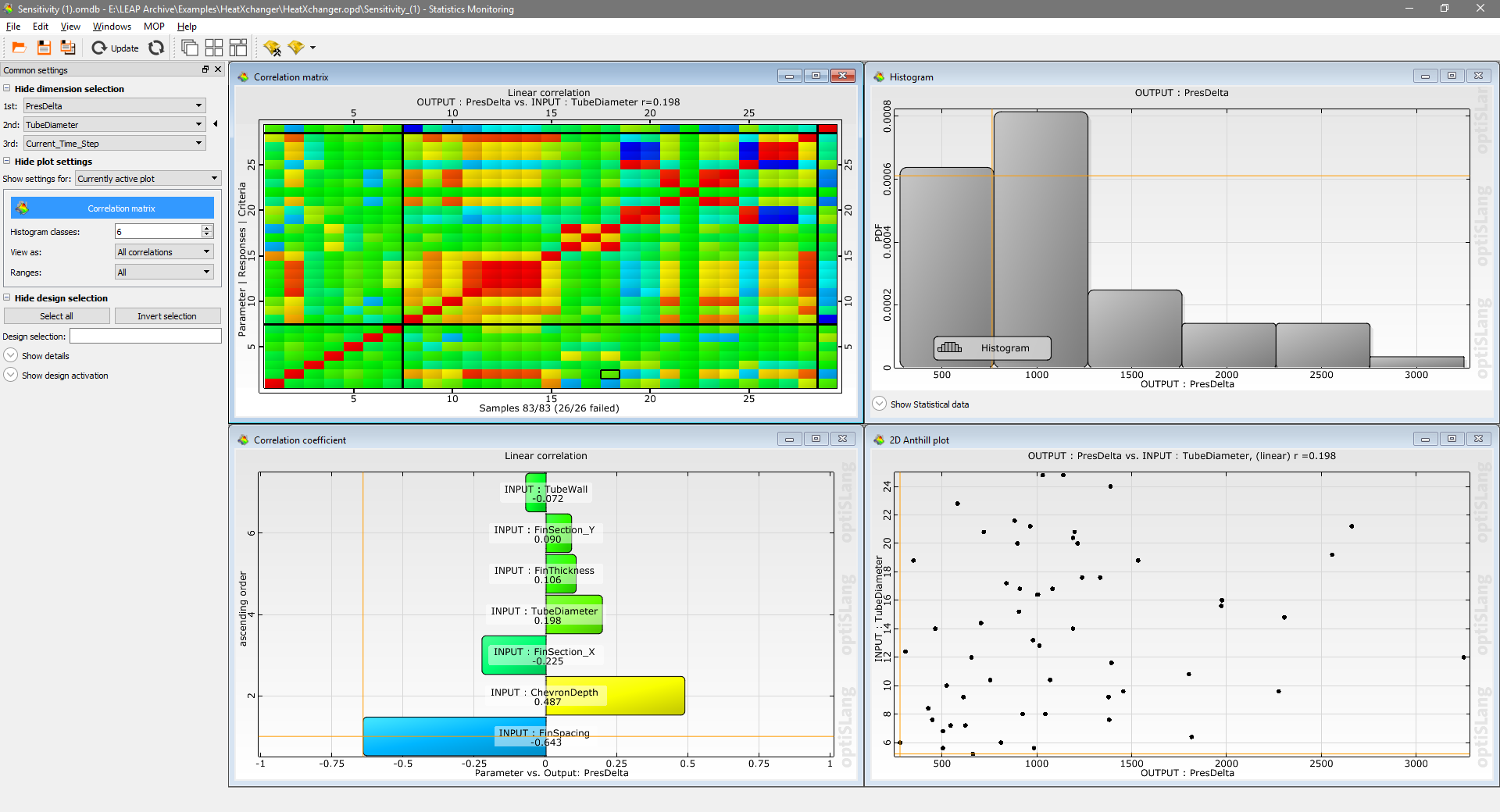
Most computer-aided simulation techniques introduce a significant amount of variation into the output of the simulation because of the mesh used to solve the problem. This is a problem across all of the different physics areas and can easily obscure any smaller improvements in the overall design. ANSYS optiSLang introduces a measure called the Coefficient of Prognosis (CoP) which is significantly less sensitive to this variation and strongly resists the tendency which existing tools have to include this noise in the final performance prediction.
With a precise and reliable measure of the relations between input/output, input/input and output/output combinations, we can now afford to under-sample the design space. Existing sensitivity studies require each input variable to be simulated in isolation from all other inputs, resulting in a configuration known as Full Factorial Sampling. Taking a minimum of 3 samples per input parameter, a design with 7 input variables would require 2187 different solutions to characterise the design space. If the simulation is nonlinear then the number of samples increases further. ANSYS optiSLang has several different sampling techniques but recommends a Hypercube sampling technique for large numbers of variables because it allows for multiple input variables to be changed simultaneously. The relations described previously can still be determined with significantly fewer sample points. A nonlinear problem with 7 variables can be characterised with just 50 simulations in some cases.
Metamodel Characterisation and Optimisation
Combining these two advances allows us to achieve the first half of the question by accurately quantifying the contribution of each input parameter and eliminating all that don’t contribute. As part of the process of analysing and eliminating parameters, a metamodel was created to represent the performance of the device. The ANSYS optiSLang environment retains this model to allow for optimisation directly on the metamodel rather than executing a simulation at each iteration. This reduces the time taken for each optimisation iteration from minutes or hours to less than a second in most cases. Tens of thousands of design points can be executed to explore the entire design space before optimising to a precise minimum, saving days in simulation time while being able to expand the possible search space many times over.
Example - Optimising a Water-Air Heat Exchanger
Heat exchangers have a lot of variables relating to the geometry of the fins, tubes and overall configuration, all of which can be adjusted to suit a combination of environment and performance target. The design constraints for this design are listed in Table 1.
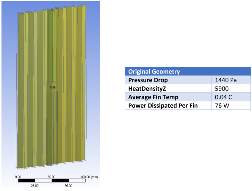
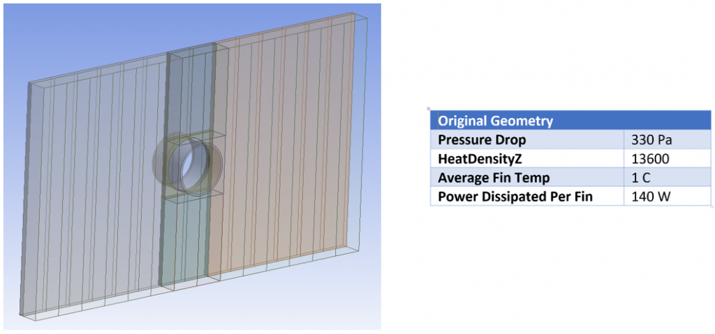
The design in Figure 2 was built within the ANSYS Workbench environment and solved with the ANSYS CFX solver. The goal is to optimise the geometry to balance maximising heat transfer while minimising pressure loss across the heat exchanger. The standard geometry configuration takes approximately 16 minutes to solve on 4 cores and 90 simulations can be completed in a 24-hour period.
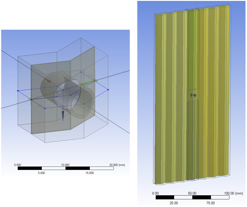
Figure 2 - The heat exchanger fin to be optimised (R). A close-up of the interface between water tube and fin as well as the cross-section of the fin (L)
Integrating ANSYS Workbench into ANSYS optiSLang
ANSYS optiSLang can interface with ANSYS Workbench in a number of different ways. In this example, optiSLang will call the Workbench project and request several simulation runs before continuing in the optiSLang environment. The results are collected by the Sensitivity system within optiSLang and further postprocessing is executed to generate characteristic performance values for each variation. If the performance formulas should change after the simulation has been completed, optiSLang will update the sensitivity study from the stored outputs without having to rerun the original simulations.
The Solver wizard within optiSLang automatically imports the input and output parameters for the project. Creating a sensitivity study or optimisation workflow then calls the template to drive Workbench rather than requiring a solver setup each time. The initial parameter limits can also be set during this wizard and referenced by each subsequent system.
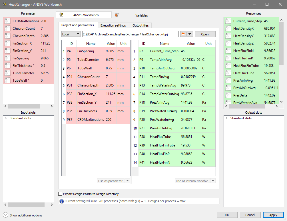
Figure 3 - Automated wizard for collecting both the input parameters and output results from the ANSYS Workbench project
Sensitivity studies can take a significant period of simulation time so optiSLang exposes its extensive sensitivity and metamodel tools to the user from the very first iteration. This allows the use to track the progress of the study and analyse trends in the results as the study progresses. Any problems with the simulation can be observed as soon as they occur rather than waiting for hours or days of simulation to complete.
Metamodel Generation
The metamodel (MOP) aims to predict as much of the variation in the measured results as possible. A table is generated which displays how much of the variation in the result is accounted for by each input variable and for the total model (Figure 5). In this example, we are also tracking values for the imposed boundary conditions (input temperatures and output pressures). The solver attempts to impose these values at the boundary of the cells so all of the variation between runs should be comprised of solver noise. This results in a very poor total value but this is expected and the output values are only used to ensure the simulation is working correctly.
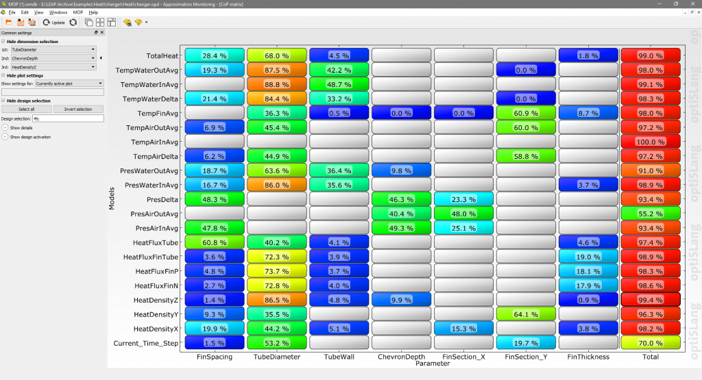
Figure 5 - Display of variation accounted for by the metamodel with respect to the input variables. This model very closely accounts for the observed variation across almost all of the measured values

Figure 6 – The response surface tool is very useful for observing the interaction between parameters and checking the metamodel for accuracy across the parameter range
Multi-Objective and Single Objective Optimisation
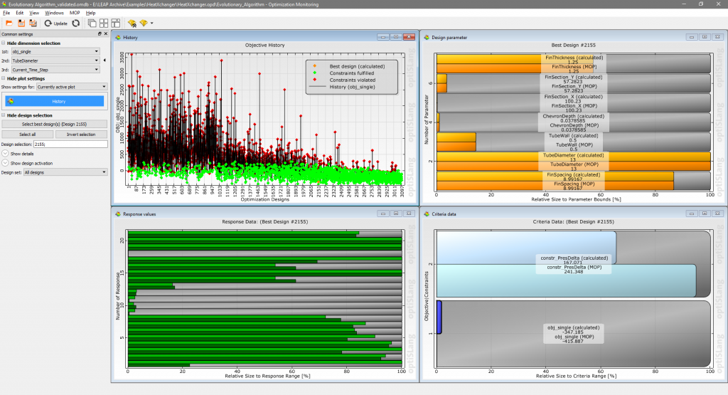
Rather than running an optimisation algorithm directly on the Workbench project, the optimisation routine can be run on the MOP itself within optiSLang. Each iteration of the MOP solver takes a fraction of a second compared to 16 minutes for the CFD run so thousands of runs are computationally inexpensive for exploring the performance envelope. This design has two objectives to be optimised towards and at this stage the trade-off between the two objectives is not well understood. Multi-objective Optimisation is possible using an Evolutionary Algorithm to search the entire design space and the resulting performance envelope can be visualised as a Pareto Front as shown in Figure 7.
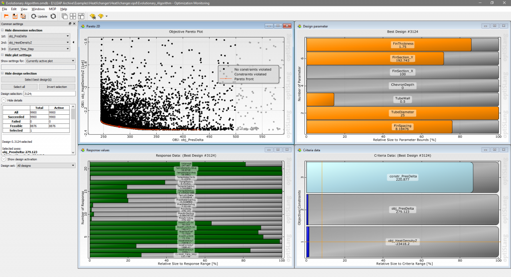
Figure 7 - Multi-Objective Optimisation in optiSLang showing the Pareto Front in red (top left plot)
Based on the shape of the Pareto Front, there is a trend towards gradually increasing static pressure for an improvement in the heat dissipation density between 250 Pa and 350 Pa. To create an effective cost function the two unit systems need to be normalised and then the function biased to prioritise each component. Then the cost function can be combined with the constraints to perform a single objective optimisation.
The sensitivity study showed an improvement in performance with an increase in the TubeDiameter and a decrease in FinSectionX. Taking the extremes of both of these parameters causes an invalid mesh because of the current constraints. So the optimiser is artificially limited to a maximum TubeDiameter of 13 mm to ensure a manufacturable design. The optimiser also automatically calls the original solver template to validate the predicted design.
The complete optimisation routine took approximately 85 minutes including the final validation run. More than 14,000 different designs were assessed in that period to produce the final design.
The optimised geometry shows a dramatic improvement in performance across all of the key metrics. If the analysis were to be run without optiSLang, the total run time would be 156 days. The total run time with optiSLang was 23 hours or 160x faster. This is in addition to the engineering knowledge gained through the sensitivity and metamodelling process which is considerable and produces significant gains in the long term. ANSYS optiSLang is the next generation in design exploration, optimisation and robustness tools.


